Automated identification of different crystal structures through unsupervised learning

Automated identification of different crystal structures through unsupervised k-means clustering

Github

Overview

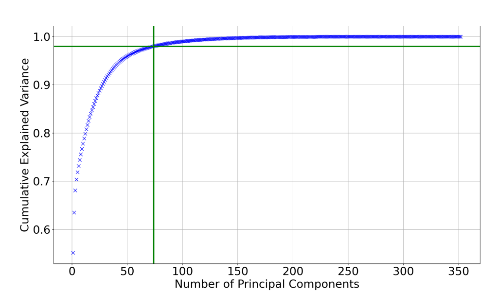
The following scripts allow for an unsupervized selection of the most distinct structures (atomic configurations) according to the clustering method of k-means applied on the CrystalNN+Average_mass_element_differences_+Average_bond_length+RDF fingerprint. Such each fingerprint uniquely characterize each structure. Prior to clustering, Principal Component Analysis (PCA) is applied to reduce the dimensionality of the fingerprint, retaining only the components that account for up to 98% of the total cumulative explained variance. These PCA-reduced components are then used for the k-means clustering process. This approach can be beneficial for example for selecting structures with the most distinct local atomic environments from a vast collection of structures generated randomly, such as through snapshots from Molecular Dynamics (MD) simulations or by other methods, like Atomsk. Identifying these unique structures can be useful for subsequent Density Functional Theory (DFT) calculations. The data obtained from DFT can then be employed to develop or improve an interatomic potential, avoiding the computational expense of examining the entire set of generated structures, which may include redundant information.

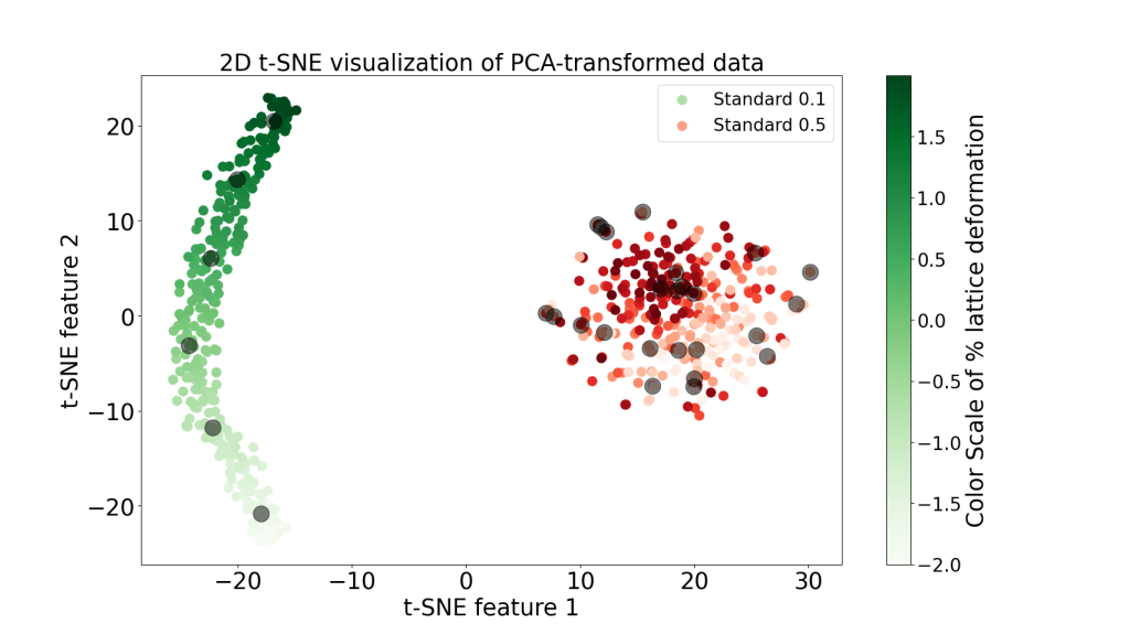
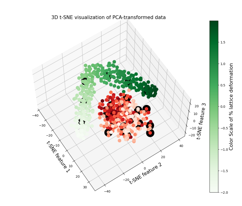
Additionally, the t-SNE method can be applied to convert the fingerprints into 2D or 3D space, enabling visualization of potential underlying patterns within the structures.

Since the CrystalNN method is applied, this selection approach is suitable only for periodic structures without a vacuum. For clustering configurations that include a vacuum, it is advisable to replace the CrystalNN method with alternatives, such as the SOAP (Smooth Overlap of Atomistic Positions) descriptor.

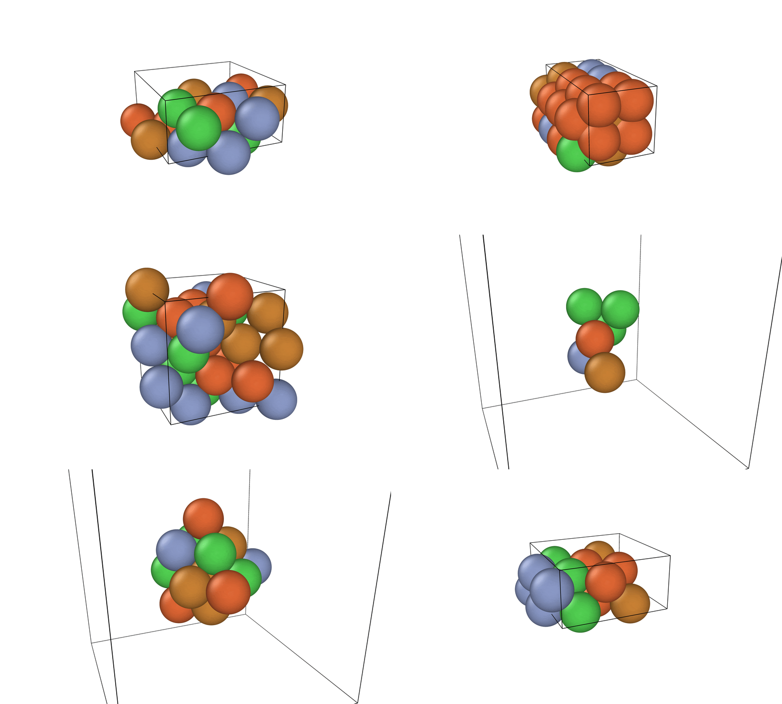
Dependencies

Python 3.x
ruamel.yaml version 0.17.40. Matminer gives errors for ruamel versions >= 0.18.x
pymatgen
matminer
numpy
sklearn
scipy
pickle
matplotlib

There are total 3 usable python scripts. The first script (featurizer.py, it employs function defined in fingerprint_calculator.py) scans crystal structures in POSCAR format within a given folder, calculates their corresponding fingerprints, and export the results in the form of dictionary into a file. These files are loaded in the second script (kmeans_loop.py), united into a one single dictionary (forming a database), and all the fingerprints are clustered by using k-means. The names of the most different structures found according to this algorithm are determined by selecting one structure from each cluster closest to its centroid. These names are then saved into an output file. For the k-means algorithm, it is necessary to determine the number of clusters (number of structures that will be selected), i.e., user must set the number of different structures he wish to select. The thirds script (kmeans_one_plot.py) can be used for the visualization of the data in terms of PCA-analysis and t-SNE method converting the fingerprints into 2D and 3D space to possibly see patterns within the structural dataset.

Workflow:

Step 1: Preparation

Prepare a folder containing the POSCAR structures

Step 2: Fingerprint Calculation

Run the „featurizer.py“ to obtain a dictionary where each structure name (key) is associated with its corresponding fingerprint (value).
1. In this script, set the correct path to the POSCAR structures (variable input_folder) and desired name of the output dictionary file (variable output_name_dictionary)
2. If the elements that are present in the clustered POSCAR files are not already in the variable chem_info2, add them with their corresponding atomic masses in amu units there.

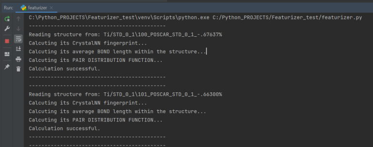
When correctly running this script, the output in the console should look like this:

Step 3: Structure Clustering

Run the following clustering script to unsupervisly identify the most distinct structures:
- „kmeans_loop.py“ for k-means-based clustering.

Notes:

Great reading about the CrystalNN method: https://docs.materialsproject.org/methodology/materials-methodology/related-materials

Matminer featurizer overview: https://hackingmaterials.lbl.gov/matminer/featurizer_summary.html

Description of the used fingerprint characterizing each atomic configuration

Each structure is characterized by the fingerprint vector comprises 352 elements, distributed as follows:

CrystalNN elements (244 Total):
- Generated by CrystalNN (61-dimensional vector for each atomic site in a structure).
- Statistical measures perform over all atomic sites within a crystal, giving: mean, standard deviation, minimum, and maximum values, thus resulting in total of 244 elements (61 × 4 statistical measures).
- CrystalNN is specifically designed for periodic structures that do not contain any vacuum. If applied to molecules, clusters, and surfaces where CrystalNN leads to errors in computation, all components of the CrystalNN part are assigned a value of zero.
Atomic mass difference elements (4 Total):
- Represents the aggregate differences in atomic masses between each atom and its nearest neighbors.
- These values are averaged over each atomic site within a crystal, giving total of 4 vector elements (mean, standard deviation, minimum, and maximum value).
- This allows to recognize structures that differ in atomic composition.
Average bond distance (4 Total) and Radial distribution function Elements (RDF, 100 Total):
- Statistics over averaged bond distance between all atomic pairs within a structure, giving total of 4 vector elements (mean, standard deviation, minimum, and maximum value).
- A radial distribution function (RDF) calculated and averaged across all atomic sites.
- The distance cutoff for the RDF is set to 10 Å.
- The RDF primarily distinguish between structures which have completely same geometrical atomic environments and the composition, but they differ in lattice parameter.
- ! Important note ! The determination of a structure’s distinctiveness is influenced by the number of points within the Radial Distribution Function (RDF). This can be adjusted in the following line:
  self.GRDF = GeneralizedRadialDistributionFunction.from_preset(‚gaussian‘, width=0.1, spacing=0.1, cutoff=10, mode=‚GRDF‘) Altering the width and spacing parameters affects the RDF’s granularity. For instance, setting width=1 and spacing=1 yields an RDF with only 10 points. Such a configuration might not be sufficient to distinguish structures that vary by deformations of up to approximately 10%. Conversely, reducing these parameters increases the RDF’s importance, enabling the identification of structures with smaller differences in their lattice parameters. You might want to tweak these parameters depending how important is for you to select as different structure .

The fingerprint consists of the following elements (352):

mean wt CN_1, std_dev wt CN_1, minimum wt CN_1, maximum wt CN_1, mean sgl_bd CN_1, std_dev sgl_bd CN_1, minimum sgl_bd CN_1, maximum sgl_bd CN_1
mean wt CN_2, std_dev wt CN_2, minimum wt CN_2, maximum wt CN_2, mean L-shaped CN_2, std_dev L-shaped CN_2, minimum L-shaped CN_2, maximum L-shaped CN_2, mean water-like CN_2, std_dev water-like CN_2, minimum water-like CN_2, maximum water-like CN_2, mean bent 120 degrees CN_2, std_dev bent 120 degrees CN_2, minimum bent 120 degrees CN_2, maximum bent 120 degrees CN_2, mean bent 150 degrees CN_2, std_dev bent 150 degrees CN_2, minimum bent 150 degrees CN_2, maximum bent 150 degrees CN_2, mean linear CN_2, std_dev linear CN_2, minimum linear CN_2, maximum linear CN_2
mean wt CN_3, std_dev wt CN_3, minimum wt CN_3, maximum wt CN_3, mean trigonal planar CN_3, std_dev trigonal planar CN_3, minimum trigonal planar CN_3, maximum trigonal planar CN_3, mean trigonal non-coplanar CN_3, std_dev trigonal non-coplanar CN_3, minimum trigonal non-coplanar CN_3, maximum trigonal non-coplanar CN_3, mean T-shaped CN_3, std_dev T-shaped CN_3, minimum T-shaped CN_3, maximum T-shaped CN_3
mean wt CN_4, std_dev wt CN_4, minimum wt CN_4, maximum wt CN_4, mean square co-planar CN_4, std_dev square co-planar CN_4, minimum square co-planar CN_4, maximum square co-planar CN_4, mean tetrahedral CN_4, std_dev tetrahedral CN_4, minimum tetrahedral CN_4, maximum tetrahedral CN_4, mean rectangular see-saw-like CN_4, std_dev rectangular see-saw-like CN_4, minimum rectangular see-saw-like CN_4, maximum rectangular see-saw-like CN_4, mean see-saw-like CN_4, std_dev see-saw-like CN_4, minimum see-saw-like CN_4, maximum see-saw-like CN_4, mean trigonal pyramidal CN_4, std_dev trigonal pyramidal CN_4, minimum trigonal pyramidal CN_4, maximum trigonal pyramidal CN_4
mean wt CN_5, std_dev wt CN_5, minimum wt CN_5, maximum wt CN_5, mean pentagonal planar CN_5, std_dev pentagonal planar CN_5, minimum pentagonal planar CN_5, maximum pentagonal planar CN_5, mean square pyramidal CN_5, std_dev square pyramidal CN_5, minimum square pyramidal CN_5, maximum square pyramidal CN_5, mean trigonal bipyramidal CN_5, std_dev trigonal bipyramidal CN_5, minimum trigonal bipyramidal CN_5, maximum trigonal bipyramidal CN_5
mean wt CN_6, std_dev wt CN_6, minimum wt CN_6, maximum wt CN_6, mean hexagonal planar CN_6, std_dev hexagonal planar CN_6, minimum hexagonal planar CN_6, maximum hexagonal planar CN_6, mean octahedral CN_6, std_dev octahedral CN_6, minimum octahedral CN_6, maximum octahedral CN_6, mean pentagonal pyramidal CN_6, std_dev pentagonal pyramidal CN_6, minimum pentagonal pyramidal CN_6, maximum pentagonal pyramidal CN_6
mean wt CN_7, std_dev wt CN_7, minimum wt CN_7, maximum wt CN_7, mean hexagonal pyramidal CN_7, std_dev hexagonal pyramidal CN_7, minimum hexagonal pyramidal CN_7, maximum hexagonal pyramidal CN_7, mean pentagonal bipyramidal CN_7, std_dev pentagonal bipyramidal CN_7, minimum pentagonal bipyramidal CN_7, maximum pentagonal bipyramidal CN_7
mean wt CN_8, std_dev wt CN_8, minimum wt CN_8, maximum wt CN_8, mean body-centered cubic CN_8, std_dev body-centered cubic CN_8, minimum body-centered cubic CN_8, maximum body-centered cubic CN_8, mean hexagonal bipyramidal CN_8, std_dev hexagonal bipyramidal CN_8, minimum hexagonal bipyramidal CN_8, maximum hexagonal bipyramidal CN_8
mean wt CN_9, std_dev wt CN_9, minimum wt CN_9, maximum wt CN_9, mean q2 CN_9, std_dev q2 CN_9, minimum q2 CN_9, maximum q2 CN_9, mean q4 CN_9, std_dev q4 CN_9, minimum q4 CN_9, maximum q4 CN_9, mean q6 CN_9, std_dev q6 CN_9, minimum q6 CN_9, maximum q6 CN_9
mean wt CN_10, std_dev wt CN_10, minimum wt CN_10, maximum wt CN_10, mean q2 CN_10, std_dev q2 CN_10, minimum q2 CN_10, maximum q2 CN_10, mean q4 CN_10, std_dev q4 CN_10, minimum q4 CN_10, maximum q4 CN_10, mean q6 CN_10, std_dev q6 CN_10, minimum q6 CN_10, maximum q6 CN_10
mean wt CN_11, std_dev wt CN_11, minimum wt CN_11, maximum wt CN_11, mean q2 CN_11, std_dev q2 CN_11, minimum q2 CN_11, maximum q2 CN_11, mean q4 CN_11, std_dev q4 CN_11, minimum q4 CN_11, maximum q4 CN_11, mean q6 CN_11, std_dev q6 CN_11, minimum q6 CN_11, maximum q6 CN_11
mean wt CN_12, std_dev wt CN_12, minimum wt CN_12, maximum wt CN_12, mean cuboctahedral CN_12, std_dev cuboctahedral CN_12, minimum cuboctahedral CN_12, maximum cuboctahedral CN_12, mean q2 CN_12, std_dev q2 CN_12, minimum q2 CN_12, maximum q2 CN_12, mean q4 CN_12, std_dev q4 CN_12, minimum q4 CN_12, maximum q4 CN_12, mean q6 CN_12, std_dev q6 CN_12, minimum q6 CN_12, maximum q6 CN_12
mean wt CN_13, std_dev wt CN_13, minimum wt CN_13, maximum wt CN_13
mean wt CN_14, std_dev wt CN_14, minimum wt CN_14, maximum wt CN_14
mean wt CN_15, std_dev wt CN_15, minimum wt CN_15, maximum wt CN_15
mean wt CN_16, std_dev wt CN_16, minimum wt CN_16, maximum wt CN_16
mean wt CN_17, std_dev wt CN_17, minimum wt CN_17, maximum wt CN_17
mean wt CN_18, std_dev wt CN_18, minimum wt CN_18, maximum wt CN_18
mean wt CN_19, std_dev wt CN_19, minimum wt CN_19, maximum wt CN_19
mean wt CN_20, std_dev wt CN_20, minimum wt CN_20, maximum wt CN_20
mean wt CN_21, std_dev wt CN_21, minimum wt CN_21, maximum wt CN_21
mean wt CN_22, std_dev wt CN_22, minimum wt CN_22, maximum wt CN_22
mean wt CN_23, std_dev wt CN_23, minimum wt CN_23, maximum wt CN_23
mean wt CN_24, std_dev wt CN_24, minimum wt CN_24, maximum wt CN_24
mean atomic_mass local diff, std_dev atomic_mass local diff, minimum atomic_mass local diff, maximum atomic_mass local diff
mean average_pair_atomic_distance, std_dev average_pair_atomic_distance, minimum average_pair_atomic_distance, maximum average_pair_atomic_distance
Gaussian center=0.0 width=0.1, Gaussian center=0.1 width=0.1, Gaussian center=0.2 width=0.1, ...,  Gaussian center=9.9 width=0.1

Python script for the k-means clustering: kmeans_loop.py

Overview

This Python script clusters a collection of crystal structures represented by their fingerprints. It uses k-means clustering to group structures based on their fingerprints. At the beginning of the script, standardization of the fingerprints is performed so that each feature is rescaled to have a mean of 0 and a standard deviation of 1 (using StandardScaler in sklearn.preprocessing). The script generates files containing lists of names for the most distinct structures identified by this algorithm.

Usage instructions

Define the number of clusters (i.e., the number of structures to select as most distinct ones) for the k-means algorithm (variable num_clusters) and the number of files to generate with the selected structures (variable how_many_files_to_generate).

Note: If you want to select a small number of structures, e.g., 5, each file will likely contain the same 5 structures. For a larger number of structures,

the selected structures may differ, as the initial positions of the centroids in k-means are determined randomly.

Possibly change weights for the individual parts of the total fingerprint. CrystalNN has 244 elements,

then 4 elements for difference in local atomic masses, 4 elements for average bond distances, and 100 elements for RDF up to 10 A.

The preselected weights are as follows:

weight_crystalNN = 1

weight_element_mass_difference = 4

weight_average_bond_distnace = 2

weight_RDF = 1

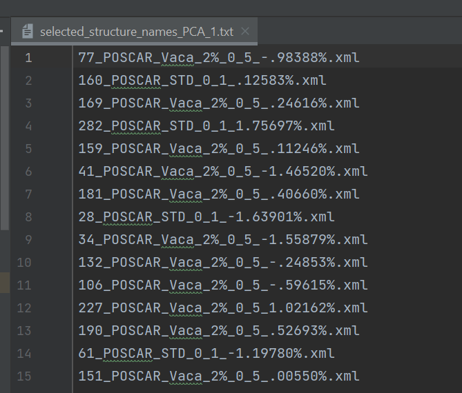
Write the names of .pkl dictionaries that were previously generated by the „featurizer.py“ and which you want to union in one database into list_files variable. Also add the corresponding names of this dictionaries in the same order into the list_of_files_names variable.
At the same folder where this script is placed, generated files with the list of selected names of structures will be saved. The name of these files will be: selected_structure_names_PCA_0.txt, selected_structure_names_PCA_1.txt, …, up to the number set in the variable how_many_files_to_generate.

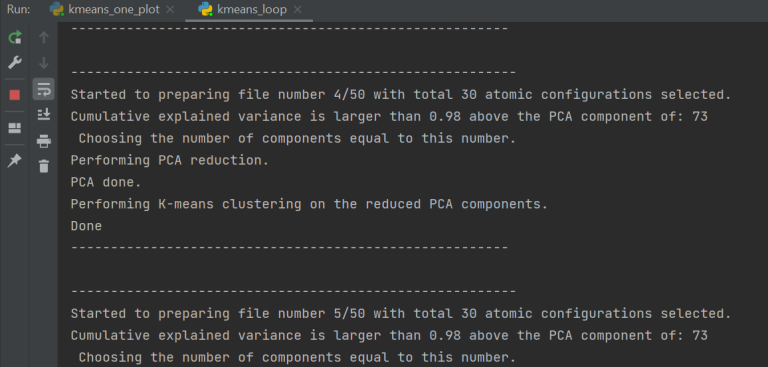
When running correctly, the console should look like this:

Example of the output file selected_structure_names_PCA_1.txt:

Python script for the visualization: kmeans_one_plot.py

Overview

This script performs clustering similar to the previous script, but only runs the process once. It then generates 4 charts to visualize the data, see examples below.

Usage instructions

Define the number of clusters (i.e., the number of structures to select) for the k-means algorithm (variable num_clusters).

Possibly change weights for the individual parts of the total fingerprint. CrystalNN has 244 elements,

then 4 elements for difference in local atomic masses, 4 elements for average bond distances, and 100 elements for RDF up to 10 A.

The preselected weights are as follows:

weight_crystalNN = 1

weight_element_mass_difference = 4

weight_average_bond_distnace = 2

weight_RDF = 1

Write the names of .pkl dictionaries that were previously generated by the „featurizer.py“ and which you want to union in one database into list_files variable. Also add the corresponding names of this dictionaries in the same order into the list_of_files_names variable

Example:

Application on 600 Ti structures (download the structures at Github in Examples/Ti folder):

300 titanium (Ti) structures with 36 atoms per supercell, a maximum atomic displacement of 0.1 Å, and lattice deformations in the range of -2% to 2% (STD_0_1).
300 titanium (Ti) structures with 36 atoms per supercell, a maximum atomic displacement of 0.5 Å, and lattice deformations in the range of -2% to 2% (STD_0_5).

1. Chart illustrating the contribution of each feature in the initial 352-element fingerprints to the 98 % of the total cumulative explained variance. For each feature, this contribution is represented by the sum of the squared loadings across all PCA components that account for 98 % of the total cumulative explained variance.

2. Chart illustrating the cumulative explained variance as a function of number of principal components.

3. Charts illustrating the t-SNE method applied on the PCA-reduced fingerprints and converting them into 2D and 3D space in order to see possible underlying patterns between the structures. The black circles highlight the 30 most distinct structures selected from a total of 600 configurations.

How k-means works here

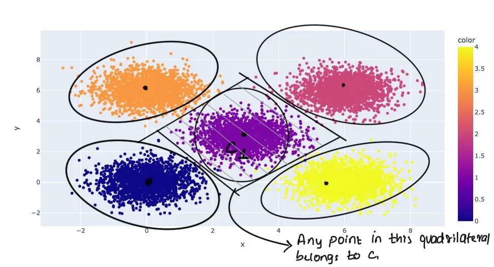
K-means clustering groups structures into distinct clusters, each containing structures with similar fingerprints. To pinpoint unique structures, a practical strategy is to select a representative structure from each cluster. Ideally, this representative should be the structure closest to the cluster’s centroid. It’s important to note that these centroids are conceptual averages of the fingerprints within a cluster and not actual structures. By choosing the structure nearest to each centroid, we are likely to identify the most distinctive structures. This is because the centroids themselves, being averages, tend to be the most divergent points among the clusters.

k-means algorithm

Initialization:
- Select K Centers: The first step is to initialize K centroids (centers of clusters). This can be done randomly or by using heuristic methods.
Assignment Step:
- Assign Data Points to Closest Centroid: Each data point in the dataset is assigned to the nearest centroid. The „nearest“ is typically determined using a distance metric like Euclidean distance. After this step, each centroid has a group of data points associated with it, forming clusters.
Update Step:
- Recalculate Centroids: After all data points are assigned to clusters, the positions of the centroids are recalculated. This is typically done by taking the mean of all points in each cluster. The centroid moves to the average position, which ideally minimizes the intra-cluster variance.
Iterative Process:
- Repeat Assignment and Update: The assignment and update steps are repeated iteratively. With each iteration, the centroids shift to more optimal positions, and data points might get reassigned to different clusters.
- Convergence: This process continues until a stopping criterion is met. Common stopping criteria include no (or minimal) change in centroids‘ positions between iterations, no (or minimal) change in points‘ assignment to clusters, or reaching a maximum number of iterations.
Result:
- Cluster Formation: The algorithm ultimately partitions the data into K clusters, each represented by its centroid. Every data point is assigned to the cluster of its nearest centroid.
- Evaluation Metrics: Various metrics, such as the Silhouette Score or Davies-Bouldin Index, can be used to evaluate the quality of clustering. These metrics assess factors like cluster compactness and separation from other clusters.